Edward Jaeck, Vice President of Strategic Growth and Business Development, Lowell Inc.09.17.19
Applying automation to data analysis is invaluable. It speeds up repetitive manual analysis, and reduces defects created by data integrity errors as well as simple errors made by the analyst. In addition, it creates standard work, which is easier to audit and train to. While not all data sets behave perfectly, there are several layers of criteria that can be applied to help automate data analysis.
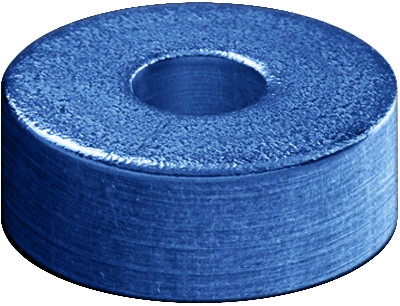
Figure 1: Image of round component with four critical dimensions. All images, tables, and graphs courtesy of Lowell Inc.
Current Situation
Currently, many original equipment manufacturers (OEMs) and contract manufacturers use Minitab for their statistical data analysis. While Minitab is a very powerful tool for data analysis, without macros, it can be cumbersome to do the same analysis with coherent summaries for large datasets in a standard-work manner. For example, imagine working with a round component as presented in Figure 1. It is a relatively simple component with four critical dimensions, which are on display in Table 1.
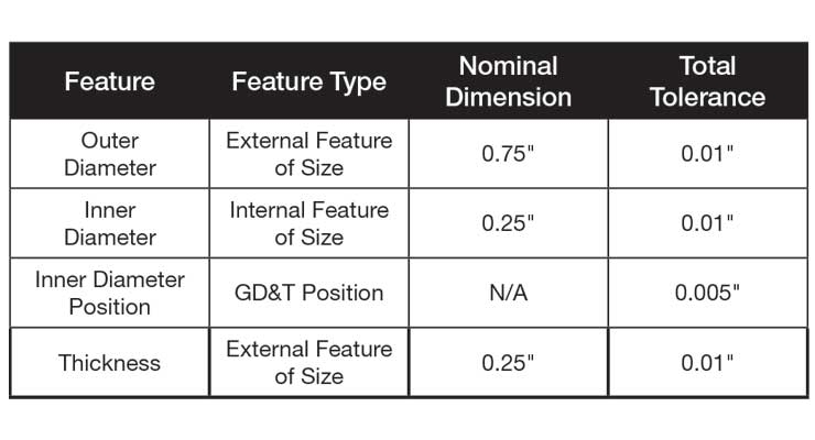
Table 1: Table of the four critical features of the component in Figure 1 with nominal dimensions and tolerances.
Now, imagine a customer wants its supplier to complete Operational Qualification (OQ) and Performance Qualification (PQ) for this component. For the OQ, the customer has insisted on three lots identified as High, Low, and Nominal. For the PQ, the customer has insisted on running three lots with each lot being run on a separate day, shift, operator, and, if possible, material batches. Assuming there are four critical features in the washer component, there will be four dimensions for OQ High, four for OQ Low, and four for OQ Nominal. In addition, there will be four for PQ1, PQ2, and PQ3. If there was just one data point for each dimension in each lot, a very simple data collection template would suffice (Table 2).
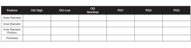
Table 2: Validation table showing OQ and PQ as separate columns.
In industry, N=1 data point per feature for OQ and PQ is never collected. The sample size is always greater than that, and in the orthopedic industry, sample size is often N=30. Once there is more than N=1 data point per lot, Table 2 would need to be altered, as the rows become the data, the number of columns increases, and the labels change.
For example, for outer diameter (OD), there would need to be six columns—OD OQ High, OD OQ Low, OD OQ Nominal, OD PQ1, OD PQ2, and OD PQ3. Following the same logic, the same six columns would be required for inner diameter (ID), inner diameter position (IDTP), and thickness (THK). Simply, there are four features in each of six validation lots (4*6=24 columns of data). Once the columns are labeled in Minitab, the data analysis can commence. Key inputs for each of the four variables are the specification limits. For OD, ID, and THK, two-sided spec limits can be expected; for the IDTP, an upper spec limit only can be expected. Once the spec limits are known, the process of checking assumptions, analyzing the data, and copying and pasting the results to a summary table can begin. An example of a completed data collection template is presented in Table 3.
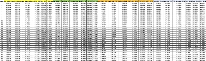
Table 3: Updated validation table with twenty-four columns and thirty rows of data for each lot-feature.
Problem Statement
Those who have used Minitab to perform data analysis know it begins as a “fun” exercise. You are immersed into the data, are able to manipulate it, tease patterns out of it, and learn more about the process. Unfortunately, that enjoyment may only last an hour or less before the experience becomes monotonous. Typing in spec limits over and over again, making the same plots repeatedly, cutting and pasting data to the summary table, missing digits, pasting data incorrectly, and having to redo analysis begins to affect the analyst. Not only is the task tiresome, it can also create data integrity issues while each cut and paste enables operator defects to creep in.
Luckily, there is a better process involving automation within Minitab. Using a custom macro eliminates the potential for errors in a number of ways.
Contents of a Solid Validation Data Analysis
Having performed data analysis at Fortune 500 level organizations such as Intel and Medtronic, as well as for clients of Lowell, it is understood there is a huge amount of pressure on the data analysis team to complete the protocol/report as soon as all the data has been collected. Those unfamiliar with the process simply do not have an appreciation for how detail-oriented one must be to perform this analysis correctly to ensure everyone in the organization, even potential naysayers, will be comfortable with the analysis.
Oftentimes, communications break down based on roles and priorities. Project managers may want to push things forward. R&D may support the project managers and may attempt to sugar coat the data to move it forward. Meanwhile, a conservative quality engineer or manager may think it is their job to reject the whole protocol due to a missed assumption or calculation mishap. From a new product introduction team perspective, each party is performing their role as they deem necessary—project managers are graded on hitting milestones for the project, R&D engineers evaluated on the device functioning properly and getting through design validation, and quality is assessed on the number of field complaints, recalls, and FDA findings later.
By defining a custom-automated macro that all parties agree upon, one can get all parties on board with the validation requirements and passing criteria. The success criteria for each feature in the validation plan can then be defined.
Incorporating time into the schedule for this team discussion regarding validation is a solid investment as some departments are not always aware of the requirements set forth in FDA guidelines or the company’s procedures for validations.
A great first step for any validation strategy is to create enough samples to pass an attribute sampling plan. While it may seem like overkill, re-running a validation because the first one failed is a much more significant expense. Delays to market can often be two to three times the cost in time. For those in the orthopedic space, it is common for OEMs to use 95 percent Confidence with 90 percent Coverage/Reliability (95/90) for component validations and 95 percent Confidence with 95 percent Coverage/Reliability (95/95) for packaging validations.
To pass a 95/90 sampling plan with attribute data, one would need to build N=29 samples and have C=0 number of rejects. Translated, that means one would need to build 29 parts with none of them falling outside of specifications. This is simple pass/fail data and can be continuous data that has been artificially dichotomized or it can be naturally occurring dichotomous data by nature. The beauty of powering the validation at the attribute size is it enables a very clean method to determine pass/fail for the validation. Simply put, if all of the columns have data within the spec limits, the validation passes. While this requirement may seem relatively basic, it is not. It is quite difficult to pick 29 random samples and not find one out of spec unless the underlying process is quite capable. By fabricating N=29 samples, the validation team can fall back to an attribute sample size argument should they get bogged down in the continuous data analysis.
For those companies demanding continuous data, the validation pathway usually consists of either A) confidence/coverage tolerance intervals or B) Cpk (process capability index) or Ppk (process performance index). Both options are nice in the sense they adapt for sample size and can be calculated with smaller sample sizes. Interpreting tolerance intervals is unique, but not difficult; simply take the entire tolerance interval and graph against the spec limits. If the entire tolerance interval falls within spec limits, it passes. If one end of the tolerance interval goes outside one of the spec limits, it fails. Minitab accomplishes this nicely in the tolerance interval graphic although it auto-scales and, sometimes, the user might want to rescale the x-axis to show the spec limits. One thing to note is the Minitab output in the tolerance interval graphic is still limited to three decimal places. If more decimal places are required, the user needs to click the button to store the tolerance intervals to the data worksheet then copy and paste from there.
Minitab can also be used to calculate the Cpk and Ppk for the data. Ppk is a better option in Minitab as the Cpk estimate comes from the control chart and assumes the data is in exactly perfect time order. The question then becomes “time order of what—the manufacturing, the measurement, or both?” This made more sense in the past when more continuous assembly lines were commonplace; the parts were sampled and then measured immediately to determine the state of control of the process. Now, a validation lot is run and samples are randomly selected, not labeled for time order then run in random order in the lab for measurements. With that said, the Cpk is meaningless since all one needs to do to inflate it is to rearrange some of the data to sort A-Z or Z-A. This puts similar measurements next to each other and minimizes the MR-bar, which then minimizes the estimate of the standard deviation.
To see this in action, create a random data set and calculate the Cpk via the Sixpack tool in Minitab. Next, sort the same data set A-Z, and calculate the Cpk again. The Cpk will go up because the standard deviation has gone down.
As an example, take the data for OQ High_OD and run a Sixpack with the data in the original order. With data in order of data collection, the Sixpack presented in Figure 2 is obtained. Note the Cpk is 6.52.

Figure 2: Sixpack of data in order of data collection.
Now, copy the same data and paste it into a new column, then sort the data A-Z with the sort function. Re-running the Sixpack on the sorted data will yield the results presented in Figure 3. Note Cpk is now over 50.24. Create some random data and try this yourself. Once you do, you will see the importance of labeling units to the unit-level in time order or skipping Cpk completely and using Ppk in Minitab.
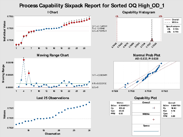
Figure 3: Sixpack on sorted data.
As can be seen in Figures 2 and 3, the Ppk remains consistent at 5.79. It is the same because the standard deviation used in the Ppk is the overall standard deviation; sorting the data has no effect.
Key Aspects of a Validation Summary Report
One key assumption for both the tolerance intervals and Ppk calculation is normality. In Minitab, this is easily accomplished with the Anderson-Darling test or the Ryan-Joyner test. Since this is one of the areas where things can become challenging, normality tests based on the Skewness-Kurtosis in the macro are included. To do this, the tests as outlined in Dr. Wayne Taylor’s book1, “Statistical Procedures for the Medical Device Industry,” were followed. (The book is highly recommended for those involved in this aspect of the industry.)
The logic for the validation is basic:
PQ-it Macro Logic
Now that the logic flow for the validation is understood, that logic can be put to work in the form of a macro. Much of the macro uses standard functions in Minitab; the process flow is as follows:
All the graphics are created and can be output to PowerPoint or Word for review. In addition, a set of summary tables is created in the session window, which can be cut and pasted into the final validation report. What previously took four hours for a dataset like the OQ-PQ data set in the previous example has been reduced to less than 20 minutes with a custom macro.
Conclusion
Data analysis is a key part of the medical device industry and being able to perform it accurately and efficiently is critical to the success of new products. To help accelerate the process, automation can be applied in statistical programs such as Minitab via macros. The PQ-it macro (created by Lowell Inc.) can analyze up to 200 columns of data and create the key outputs, graphics, and summary tables in PowerPoint and Word in less than 20 minutes. This represents a more than 90 percent reduction in analysis time while greatly minimizing errors.
Reference
Edward Jaeck is vice president of strategic growth and business development at Minneapolis-based Lowell Inc. He holds a bachelor’s degree in mechanical engineering and a master’s degree in industrial engineering from Arizona State University, and also a master’s degree in engineering management from the University of Colorado. Edward came to Lowell after serving in previous positions at Intel and Medtronic, where he focused on technology development, supplier development, manufacturing process development, and qualification in support of new product development. He is an ASQ member, a six-sigma black belt, and a past senior GD&T certificate holder. You can contact him at edward.jaeck@lowellinc.com.
Figure 1: Image of round component with four critical dimensions. All images, tables, and graphs courtesy of Lowell Inc.
Current Situation
Currently, many original equipment manufacturers (OEMs) and contract manufacturers use Minitab for their statistical data analysis. While Minitab is a very powerful tool for data analysis, without macros, it can be cumbersome to do the same analysis with coherent summaries for large datasets in a standard-work manner. For example, imagine working with a round component as presented in Figure 1. It is a relatively simple component with four critical dimensions, which are on display in Table 1.
Table 1: Table of the four critical features of the component in Figure 1 with nominal dimensions and tolerances.
Now, imagine a customer wants its supplier to complete Operational Qualification (OQ) and Performance Qualification (PQ) for this component. For the OQ, the customer has insisted on three lots identified as High, Low, and Nominal. For the PQ, the customer has insisted on running three lots with each lot being run on a separate day, shift, operator, and, if possible, material batches. Assuming there are four critical features in the washer component, there will be four dimensions for OQ High, four for OQ Low, and four for OQ Nominal. In addition, there will be four for PQ1, PQ2, and PQ3. If there was just one data point for each dimension in each lot, a very simple data collection template would suffice (Table 2).
Table 2: Validation table showing OQ and PQ as separate columns.
In industry, N=1 data point per feature for OQ and PQ is never collected. The sample size is always greater than that, and in the orthopedic industry, sample size is often N=30. Once there is more than N=1 data point per lot, Table 2 would need to be altered, as the rows become the data, the number of columns increases, and the labels change.
For example, for outer diameter (OD), there would need to be six columns—OD OQ High, OD OQ Low, OD OQ Nominal, OD PQ1, OD PQ2, and OD PQ3. Following the same logic, the same six columns would be required for inner diameter (ID), inner diameter position (IDTP), and thickness (THK). Simply, there are four features in each of six validation lots (4*6=24 columns of data). Once the columns are labeled in Minitab, the data analysis can commence. Key inputs for each of the four variables are the specification limits. For OD, ID, and THK, two-sided spec limits can be expected; for the IDTP, an upper spec limit only can be expected. Once the spec limits are known, the process of checking assumptions, analyzing the data, and copying and pasting the results to a summary table can begin. An example of a completed data collection template is presented in Table 3.
Table 3: Updated validation table with twenty-four columns and thirty rows of data for each lot-feature.
Problem Statement
Those who have used Minitab to perform data analysis know it begins as a “fun” exercise. You are immersed into the data, are able to manipulate it, tease patterns out of it, and learn more about the process. Unfortunately, that enjoyment may only last an hour or less before the experience becomes monotonous. Typing in spec limits over and over again, making the same plots repeatedly, cutting and pasting data to the summary table, missing digits, pasting data incorrectly, and having to redo analysis begins to affect the analyst. Not only is the task tiresome, it can also create data integrity issues while each cut and paste enables operator defects to creep in.
Luckily, there is a better process involving automation within Minitab. Using a custom macro eliminates the potential for errors in a number of ways.
Contents of a Solid Validation Data Analysis
Having performed data analysis at Fortune 500 level organizations such as Intel and Medtronic, as well as for clients of Lowell, it is understood there is a huge amount of pressure on the data analysis team to complete the protocol/report as soon as all the data has been collected. Those unfamiliar with the process simply do not have an appreciation for how detail-oriented one must be to perform this analysis correctly to ensure everyone in the organization, even potential naysayers, will be comfortable with the analysis.
Oftentimes, communications break down based on roles and priorities. Project managers may want to push things forward. R&D may support the project managers and may attempt to sugar coat the data to move it forward. Meanwhile, a conservative quality engineer or manager may think it is their job to reject the whole protocol due to a missed assumption or calculation mishap. From a new product introduction team perspective, each party is performing their role as they deem necessary—project managers are graded on hitting milestones for the project, R&D engineers evaluated on the device functioning properly and getting through design validation, and quality is assessed on the number of field complaints, recalls, and FDA findings later.
By defining a custom-automated macro that all parties agree upon, one can get all parties on board with the validation requirements and passing criteria. The success criteria for each feature in the validation plan can then be defined.
Incorporating time into the schedule for this team discussion regarding validation is a solid investment as some departments are not always aware of the requirements set forth in FDA guidelines or the company’s procedures for validations.
A great first step for any validation strategy is to create enough samples to pass an attribute sampling plan. While it may seem like overkill, re-running a validation because the first one failed is a much more significant expense. Delays to market can often be two to three times the cost in time. For those in the orthopedic space, it is common for OEMs to use 95 percent Confidence with 90 percent Coverage/Reliability (95/90) for component validations and 95 percent Confidence with 95 percent Coverage/Reliability (95/95) for packaging validations.
To pass a 95/90 sampling plan with attribute data, one would need to build N=29 samples and have C=0 number of rejects. Translated, that means one would need to build 29 parts with none of them falling outside of specifications. This is simple pass/fail data and can be continuous data that has been artificially dichotomized or it can be naturally occurring dichotomous data by nature. The beauty of powering the validation at the attribute size is it enables a very clean method to determine pass/fail for the validation. Simply put, if all of the columns have data within the spec limits, the validation passes. While this requirement may seem relatively basic, it is not. It is quite difficult to pick 29 random samples and not find one out of spec unless the underlying process is quite capable. By fabricating N=29 samples, the validation team can fall back to an attribute sample size argument should they get bogged down in the continuous data analysis.
For those companies demanding continuous data, the validation pathway usually consists of either A) confidence/coverage tolerance intervals or B) Cpk (process capability index) or Ppk (process performance index). Both options are nice in the sense they adapt for sample size and can be calculated with smaller sample sizes. Interpreting tolerance intervals is unique, but not difficult; simply take the entire tolerance interval and graph against the spec limits. If the entire tolerance interval falls within spec limits, it passes. If one end of the tolerance interval goes outside one of the spec limits, it fails. Minitab accomplishes this nicely in the tolerance interval graphic although it auto-scales and, sometimes, the user might want to rescale the x-axis to show the spec limits. One thing to note is the Minitab output in the tolerance interval graphic is still limited to three decimal places. If more decimal places are required, the user needs to click the button to store the tolerance intervals to the data worksheet then copy and paste from there.
Minitab can also be used to calculate the Cpk and Ppk for the data. Ppk is a better option in Minitab as the Cpk estimate comes from the control chart and assumes the data is in exactly perfect time order. The question then becomes “time order of what—the manufacturing, the measurement, or both?” This made more sense in the past when more continuous assembly lines were commonplace; the parts were sampled and then measured immediately to determine the state of control of the process. Now, a validation lot is run and samples are randomly selected, not labeled for time order then run in random order in the lab for measurements. With that said, the Cpk is meaningless since all one needs to do to inflate it is to rearrange some of the data to sort A-Z or Z-A. This puts similar measurements next to each other and minimizes the MR-bar, which then minimizes the estimate of the standard deviation.
To see this in action, create a random data set and calculate the Cpk via the Sixpack tool in Minitab. Next, sort the same data set A-Z, and calculate the Cpk again. The Cpk will go up because the standard deviation has gone down.
As an example, take the data for OQ High_OD and run a Sixpack with the data in the original order. With data in order of data collection, the Sixpack presented in Figure 2 is obtained. Note the Cpk is 6.52.
Figure 2: Sixpack of data in order of data collection.
Now, copy the same data and paste it into a new column, then sort the data A-Z with the sort function. Re-running the Sixpack on the sorted data will yield the results presented in Figure 3. Note Cpk is now over 50.24. Create some random data and try this yourself. Once you do, you will see the importance of labeling units to the unit-level in time order or skipping Cpk completely and using Ppk in Minitab.
Figure 3: Sixpack on sorted data.
As can be seen in Figures 2 and 3, the Ppk remains consistent at 5.79. It is the same because the standard deviation used in the Ppk is the overall standard deviation; sorting the data has no effect.
Key Aspects of a Validation Summary Report
- Ppk: This is the most common requirement for validation plans.
- Confidence/Coverage tolerance intervals: This is still very common in the medical device industry as it allows the team to pass with attribute data or continuous data.
- Actual Sample Size vs. Sample Size to pass attribute sampling plan: This is key information as we can always fall back to an attribute sample size argument if the continuous data analysis gets bogged down.
One key assumption for both the tolerance intervals and Ppk calculation is normality. In Minitab, this is easily accomplished with the Anderson-Darling test or the Ryan-Joyner test. Since this is one of the areas where things can become challenging, normality tests based on the Skewness-Kurtosis in the macro are included. To do this, the tests as outlined in Dr. Wayne Taylor’s book1, “Statistical Procedures for the Medical Device Industry,” were followed. (The book is highly recommended for those involved in this aspect of the industry.)
The logic for the validation is basic:
-
Did the dataset pass a normality test?
- If data passes normality then the standard Tolerance Interval and Ppk calculations (both assume normality) can be used.
- If the data does not pass normality tests, check for outliers and re-test, normalize the dataset, or determine if the dataset is “highly capable,”—a process to compare the Ppk estimate to a tabulated value from Dr. Taylor’s book.
- Did the validation have enough samples to pass an attribute sampling plan and were all of those samples within spec?
PQ-it Macro Logic
Now that the logic flow for the validation is understood, that logic can be put to work in the form of a macro. Much of the macro uses standard functions in Minitab; the process flow is as follows:
- Step 1: Click box for desired Confidence/Coverage required for the validation (options: 95/90, 95/95, or 95/99).
- Step 2: Check for outliers via the boxplot tool and formal outlier test for each column of data.
- Step 3: Check for normality using Anderson-Darling, Ryan-Joiner, and Skewness-Kurtosis tests for each column of data.
- Step 4: Calculate the tolerance intervals for each column of data.
- Step 5: Calculate Pp and Ppk for each column of data.
- Step 6: Calculate the actual sample size for each column of data.
All the graphics are created and can be output to PowerPoint or Word for review. In addition, a set of summary tables is created in the session window, which can be cut and pasted into the final validation report. What previously took four hours for a dataset like the OQ-PQ data set in the previous example has been reduced to less than 20 minutes with a custom macro.
Conclusion
Data analysis is a key part of the medical device industry and being able to perform it accurately and efficiently is critical to the success of new products. To help accelerate the process, automation can be applied in statistical programs such as Minitab via macros. The PQ-it macro (created by Lowell Inc.) can analyze up to 200 columns of data and create the key outputs, graphics, and summary tables in PowerPoint and Word in less than 20 minutes. This represents a more than 90 percent reduction in analysis time while greatly minimizing errors.
Reference
- Taylor, Wayne (2017). Statistical Procedures for the Medical device Industry. Taylor Enterprises, Inc.,www.variation.com.
Edward Jaeck is vice president of strategic growth and business development at Minneapolis-based Lowell Inc. He holds a bachelor’s degree in mechanical engineering and a master’s degree in industrial engineering from Arizona State University, and also a master’s degree in engineering management from the University of Colorado. Edward came to Lowell after serving in previous positions at Intel and Medtronic, where he focused on technology development, supplier development, manufacturing process development, and qualification in support of new product development. He is an ASQ member, a six-sigma black belt, and a past senior GD&T certificate holder. You can contact him at edward.jaeck@lowellinc.com.