Edward Jaeck, Vice President of Strategic Growth and Business Development, Lowell Inc.02.13.19
If your company outsources its medical device manufacturing, metrology matching analysis is a critical process for successful product design, development, and results.
Metrology matching is a process that aligns two separate inspection systems—typically your system and a supplier’s—to ensure consistent results. This matching process is essential if two firms are not measuring and inspecting products using the same equipment and test methods, which is common when outsourcing. The analysis is often driven by the medical device company or OEM, although some suppliers are also championing this process.
There are three key benefits gained by product development teams and companies who commit to metrology matching:
To better explain how metrology matching works, following is an 11-step process that can be used to gather, analyze, and align data from two separate systems. The following steps will help with the metrology matching analysis for medical device companies, OEMs, and suppliers.
11 Steps of the Metrology Matching Analysis Process
Metrology matching begins by choosing the appropriate analysis approach. Traditional regression analysis using ordinary least squares assumes all the variation is in the Y variable, with zero variation in the X variable. When comparing two measurement systems, both have variation, and because of that, orthogonal regression is the preferred analysis method as it allows for errors in both the X and Y variables.
To help explain the process, this article goes through an example with real internal case study data that has been coded and transformed to protect confidentiality. It should be noted there are multiple methods to conduct this analysis,1 but the orthogonal regression method is being utilized, which is supported on the Minitab website.2 For this case study, the part in question had three features of interest. To keep it simple, those three features will be referred to as length, width, and height.
Step 1: Locate N=30 parts covering the tolerance spread as best as possible. We did this by sorting and choosing parts that spanned the total tolerance as best we could. (Note: This is challenging if you are a precision shop, so you may need to make skew samples intentionally for the study.)
Step 2: The OEM or medical device company will define the inspection method in detail for each of the features measured. This should include the fixturing method on the machine, orientation on the machine, algorithm used on the machine, numbers of data points used in the algorithm, etc.
Step 3: Label the parts 1-30.
Step 4: Measure each of the parts 1-30 at the OEM with supplier support on site. Record the data, checking for outliers as you go. The optimal OEM team should include a representative from design, supplier quality, and the incoming inspection lab team. The optimal supplier team should include a representative from the outgoing inspection lab and the manufacturing team.
Step 5: Ship the 30 parts to the supplier and have them measure with OEM support on site. Record the data, checking for outliers as you go.
Step 6: Bring the data into one summary Excel file as in Table 1.
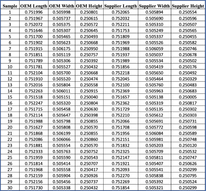
Table 1: Metrology matching data collection should be compiled into a summary Excel file.
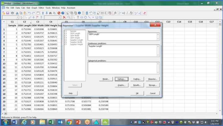
Step 7: Bring the data into Minitab and run the orthogonal regression tool. Since we are trying to predict the OEM data based on the supplier data, use the OEM data for the Y variable and the supplier data for the X variable. The orthogonal regression tool will require a number for the error variance ratio. One way to get the error variance ratio is to run a Type 1 repeatability study on each machine with one part (can be the same part or different part if needed) and 30 repetitions. With data collected, check for stability using an I-MR chart and if stable, calculate the standard deviation, square it to get the variance, then take the ratio of those variances to calculate the error variance ratio. If those variance estimates are not available, then using 1.00 as the default has been found to be acceptable as the test is somewhat robust against departures from this assumption in ranges from 0.5 to 2.3
For now, use the error variance ratio as 1.00. That should look like the table in Figure 1.
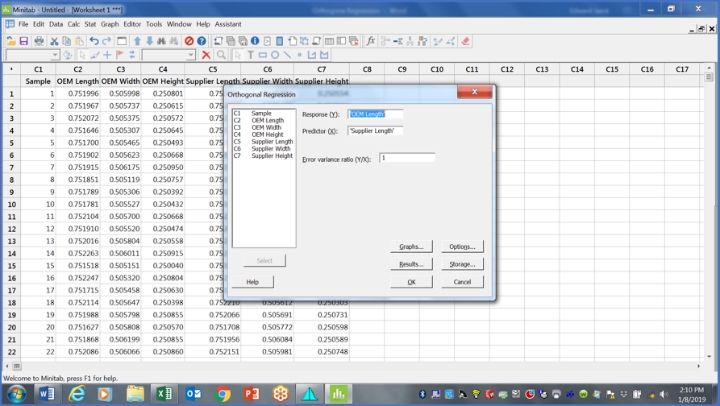
Figure 1: This table shows which variable goes where and initial guess for error variance ratio (Y/X).
Step 8: Open the graphs button and click on the Four in One button under the Residual Plots section and click OK.
Hit OK to run analysis and you will get a couple output plots (Figure 2).
The first plot is the Four in One residuals analysis plot. Use the Four in One plot to check for large residual data points or outliers as they may signal lack of fit in the model.
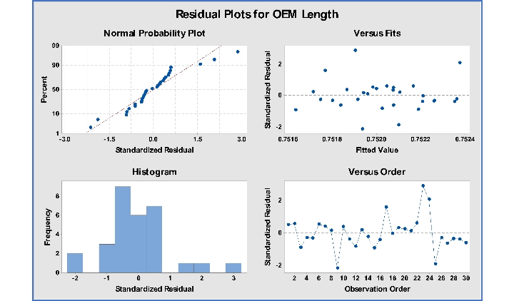
Figure 2: Four in one residual plots for OEM Length is an important part of metrology matching analysis.
The next plot (Figure 3) is a fitted line plot of the OEM data vs. supplier data and should be at a 45-degree angle if the slope is near 1.00. At the bottom of the plot is the orthogonal regression equation, which relates the supplier data to OEM data.
In this case: OEM Data=0.002+0.998*supplier data. This is the predictive equation we seek.
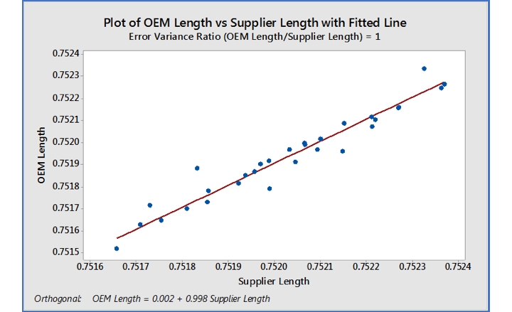
Figure 3: Fitted line plot of OEM Length vs. Supplier Length
Step 9: Review the data from the session window to interpret the results.
Item 1: The Slope=1.00 (i.e., β1=1). This checks for linearity in accuracy. (Note: reading the session window, it is the author’s opinion that the hypothesis on β1 is actually β1=0, with the alternative hypothesis being β1≠0. This is the only way to explain the inverted p-values for β0 and β1 in the Minitab blog example.) In other software, we can set β1=1 directly.
Item 2: The Y intercept=0.00 (i.e., β0=0). This checks for bias.
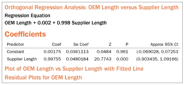
Table 2: Session window output from orthogonal regression analysis.
Decision Rules: Check the Approx. 95% Confidence Intervals (CI) from Table 2 to see if they contain their respective hypothesized value.
In the case of Item 1 (Slope=1.00), the 95% CI should contain 1.00.
In our example, the best estimate for the slope = 0.998 with its 95% CI running from 0.903 to 1.092. This includes 1.00.
In the case of Item 2 (Y-intercept=0.00), the 95% CI should contain 0.00. In our example, the best estimate for Y-intercept or the constant = 0.0018 and the 95% CI runs from -0.0690 to 0.0725, thus containing 0.00.
Matching Phase Conclusion: Both hypotheses have been satisfied, so we can consider the metrology systems matched.
Step 10: This is the correlation phase. To check for correlation, it is best to use the R2 from the orthogonal regression analysis. Since Minitab does not provide that, the best we can do is run an ordinary least squares regression analysis with the supplier data as the Continuous predictor and the OEM data as the Response or create a fitted line plot. Check the R-Sq. to see if it is greater than 75 percent. In other software, the R2 is an output in the orthogonal regression analysis and can be read directly.
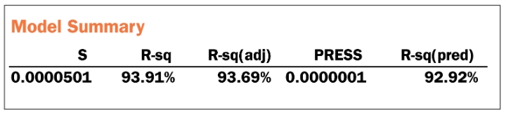
Correlation Phase Conclusion: Since the R-sq. > 75 percent, we can consider the metrology systems correlated.
Step 11: Combine results. Metrology systems are matched and correlated. No transformation is needed. Use supplier data as is at incoming inspection.
If we repeat the same process for the width, we get the following summary table, which we leave to the reader as practice.
Regression Equation
OEM Width = 0.003 + 0.994 Supplier Width
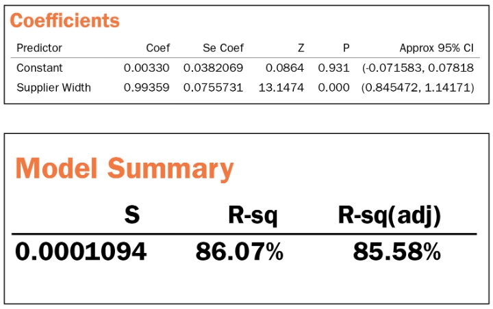
Width conclusion: Metrology matched and correlated. Use supplier data as is.
If we repeat the same process for the height, we get the following summary table, which we leave for you as practice.
Regression Equation
OEM Height = 0.006 + 0.978 Supplier Height
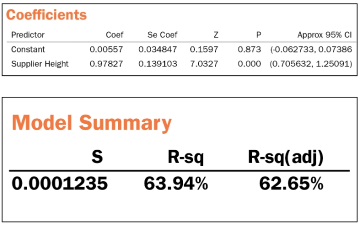
Height conclusion: Metrology matched but not correlated. More investigation needed.
Conclusion
Many medical device companies and OEMs do not invest in metrology matching, despite the tremendous information that can be learned about internal processes, supplier processes, and potential hurdles in a product’s design. By incorporating this process into product development outsourcing requirements, a company can gain key insights about design and inspection that ultimately lead to more successful outcomes.
References
1 http://bit.ly/odt190151
2 http://bit.ly/odt190150
3 Linnet, K. (1998). Performance of Deming regression analysis in case of misspecified analytical error ratio in method comparison studies. Clinical chemistry. 44. p. 1024-31.
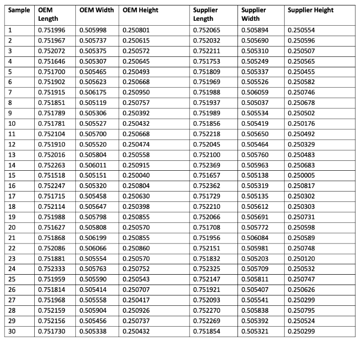
Appendix A: Raw data table for reader analysis
Edward Jaeck is vice president of strategic growth and business development at Lowell Inc. in Minnesota. He has a bachelor’s degree in mechanical engineering, a master’s degree in industrial engineering, and a master’s degree in engineering management. Prior to Lowell, Jaeck spent 12 years in various roles at Intel in Arizona and five years in new product development and quality at Medtronic in California. For more information, suggestions, or questions, contact the author at edward.jaeck@lowellinc.com.
Metrology matching is a process that aligns two separate inspection systems—typically your system and a supplier’s—to ensure consistent results. This matching process is essential if two firms are not measuring and inspecting products using the same equipment and test methods, which is common when outsourcing. The analysis is often driven by the medical device company or OEM, although some suppliers are also championing this process.
There are three key benefits gained by product development teams and companies who commit to metrology matching:
- Metrology matching accelerates the design process by drawing out key designer intentions. One of the first tasks of metrology matching is to ensure all features have been defined. Then, metrology needs to be chosen and gauge studies completed to measure the critical features. This process typically helps design teams focus on the features that really drive the product functionality—the critical features—rather than negligible details. Ideally, the matching studies occur before the design validation (DV) stage for medical devices. Conducting the matching studies prior to DV gives the design team and the management team full confidence in the DV data and, thus, paperwork submitted to the FDA.
- Metrology matching instills confidence with the medical device company that the supplier’s metrology environment and process is as good or better than their own. This improves trust, speed, and time to market. These three items help maximize the return on investment for the company.
- Metrology matching analysis is the key ingredient to all “no inspection needed” or “dock-to-stock” programs. These programs eliminate incoming inspection at the medical device company’s site, which saves money. Even if dock-to-stock programs aren’t possible for a company, conducting the matching studies upfront can resolve discrepancies in methods between a company and its supplier. This can reduce the number of returned material authorizations or false non-conforming returns.
To better explain how metrology matching works, following is an 11-step process that can be used to gather, analyze, and align data from two separate systems. The following steps will help with the metrology matching analysis for medical device companies, OEMs, and suppliers.
11 Steps of the Metrology Matching Analysis Process
Metrology matching begins by choosing the appropriate analysis approach. Traditional regression analysis using ordinary least squares assumes all the variation is in the Y variable, with zero variation in the X variable. When comparing two measurement systems, both have variation, and because of that, orthogonal regression is the preferred analysis method as it allows for errors in both the X and Y variables.
To help explain the process, this article goes through an example with real internal case study data that has been coded and transformed to protect confidentiality. It should be noted there are multiple methods to conduct this analysis,1 but the orthogonal regression method is being utilized, which is supported on the Minitab website.2 For this case study, the part in question had three features of interest. To keep it simple, those three features will be referred to as length, width, and height.
Step 1: Locate N=30 parts covering the tolerance spread as best as possible. We did this by sorting and choosing parts that spanned the total tolerance as best we could. (Note: This is challenging if you are a precision shop, so you may need to make skew samples intentionally for the study.)
Step 2: The OEM or medical device company will define the inspection method in detail for each of the features measured. This should include the fixturing method on the machine, orientation on the machine, algorithm used on the machine, numbers of data points used in the algorithm, etc.
Step 3: Label the parts 1-30.
Step 4: Measure each of the parts 1-30 at the OEM with supplier support on site. Record the data, checking for outliers as you go. The optimal OEM team should include a representative from design, supplier quality, and the incoming inspection lab team. The optimal supplier team should include a representative from the outgoing inspection lab and the manufacturing team.
Step 5: Ship the 30 parts to the supplier and have them measure with OEM support on site. Record the data, checking for outliers as you go.
Step 6: Bring the data into one summary Excel file as in Table 1.
Table 1: Metrology matching data collection should be compiled into a summary Excel file.
Step 7: Bring the data into Minitab and run the orthogonal regression tool. Since we are trying to predict the OEM data based on the supplier data, use the OEM data for the Y variable and the supplier data for the X variable. The orthogonal regression tool will require a number for the error variance ratio. One way to get the error variance ratio is to run a Type 1 repeatability study on each machine with one part (can be the same part or different part if needed) and 30 repetitions. With data collected, check for stability using an I-MR chart and if stable, calculate the standard deviation, square it to get the variance, then take the ratio of those variances to calculate the error variance ratio. If those variance estimates are not available, then using 1.00 as the default has been found to be acceptable as the test is somewhat robust against departures from this assumption in ranges from 0.5 to 2.3
For now, use the error variance ratio as 1.00. That should look like the table in Figure 1.
Figure 1: This table shows which variable goes where and initial guess for error variance ratio (Y/X).
Step 8: Open the graphs button and click on the Four in One button under the Residual Plots section and click OK.
Hit OK to run analysis and you will get a couple output plots (Figure 2).
The first plot is the Four in One residuals analysis plot. Use the Four in One plot to check for large residual data points or outliers as they may signal lack of fit in the model.
Figure 2: Four in one residual plots for OEM Length is an important part of metrology matching analysis.
The next plot (Figure 3) is a fitted line plot of the OEM data vs. supplier data and should be at a 45-degree angle if the slope is near 1.00. At the bottom of the plot is the orthogonal regression equation, which relates the supplier data to OEM data.
In this case: OEM Data=0.002+0.998*supplier data. This is the predictive equation we seek.
Figure 3: Fitted line plot of OEM Length vs. Supplier Length
Step 9: Review the data from the session window to interpret the results.
Item 1: The Slope=1.00 (i.e., β1=1). This checks for linearity in accuracy. (Note: reading the session window, it is the author’s opinion that the hypothesis on β1 is actually β1=0, with the alternative hypothesis being β1≠0. This is the only way to explain the inverted p-values for β0 and β1 in the Minitab blog example.) In other software, we can set β1=1 directly.
Item 2: The Y intercept=0.00 (i.e., β0=0). This checks for bias.
Table 2: Session window output from orthogonal regression analysis.
Decision Rules: Check the Approx. 95% Confidence Intervals (CI) from Table 2 to see if they contain their respective hypothesized value.
In the case of Item 1 (Slope=1.00), the 95% CI should contain 1.00.
In our example, the best estimate for the slope = 0.998 with its 95% CI running from 0.903 to 1.092. This includes 1.00.
In the case of Item 2 (Y-intercept=0.00), the 95% CI should contain 0.00. In our example, the best estimate for Y-intercept or the constant = 0.0018 and the 95% CI runs from -0.0690 to 0.0725, thus containing 0.00.
Matching Phase Conclusion: Both hypotheses have been satisfied, so we can consider the metrology systems matched.
Step 10: This is the correlation phase. To check for correlation, it is best to use the R2 from the orthogonal regression analysis. Since Minitab does not provide that, the best we can do is run an ordinary least squares regression analysis with the supplier data as the Continuous predictor and the OEM data as the Response or create a fitted line plot. Check the R-Sq. to see if it is greater than 75 percent. In other software, the R2 is an output in the orthogonal regression analysis and can be read directly.
Step 11: Combine results. Metrology systems are matched and correlated. No transformation is needed. Use supplier data as is at incoming inspection.
If we repeat the same process for the width, we get the following summary table, which we leave to the reader as practice.
Regression Equation
OEM Width = 0.003 + 0.994 Supplier Width
If we repeat the same process for the height, we get the following summary table, which we leave for you as practice.
Regression Equation
OEM Height = 0.006 + 0.978 Supplier Height
Conclusion
Many medical device companies and OEMs do not invest in metrology matching, despite the tremendous information that can be learned about internal processes, supplier processes, and potential hurdles in a product’s design. By incorporating this process into product development outsourcing requirements, a company can gain key insights about design and inspection that ultimately lead to more successful outcomes.
References
1 http://bit.ly/odt190151
2 http://bit.ly/odt190150
3 Linnet, K. (1998). Performance of Deming regression analysis in case of misspecified analytical error ratio in method comparison studies. Clinical chemistry. 44. p. 1024-31.
Appendix A: Raw data table for reader analysis
Edward Jaeck is vice president of strategic growth and business development at Lowell Inc. in Minnesota. He has a bachelor’s degree in mechanical engineering, a master’s degree in industrial engineering, and a master’s degree in engineering management. Prior to Lowell, Jaeck spent 12 years in various roles at Intel in Arizona and five years in new product development and quality at Medtronic in California. For more information, suggestions, or questions, contact the author at edward.jaeck@lowellinc.com.